Introduction
Variational Autoencoders (VAEs) are a powerful class of generative models that learn to compress high-dimensional data into a lower-dimensional latent space while maintaining the ability to reconstruct the original data. What makes VAEs special is their probabilistic foundation—instead of learning a deterministic mapping, they learn a distribution over latent codes, enabling both meaningful compression and generation of new samples.
Beta-VAE is an elegant extension of the standard VAE framework introduced by Higgins et al. (2016) that places more emphasis on learning disentangled representations—latent variables that capture independent, interpretable factors of variation in the data. Rather than treating all latent dimensions equally, Beta-VAE uses a weighted parameter β to encourage the model to learn factors that are more sparse and independent from one another.
Why does disentanglement matter? Disentangled representations are fundamentally more interpretable and useful. In face images, one latent dimension might exclusively represent "smiling" while another represents "age." This independence means: (1) we can understand what each dimension captures, (2) we can manipulate one factor without affecting others, and (3) representations learned from one dataset may transfer better to related tasks. This is far superior to entangled representations where a single latent code might implicitly mix together pose, lighting, expression, and identity.
What You'll Learn in This Tutorial
- The mathematical foundations of Variational Autoencoders and the evidence lower bound (ELBO)
- Why standard VAEs fail to learn disentangled representations and how Beta-VAE solves this problem
- Detailed architecture: convolutional encoders, reparameterization, and transposed convolutional decoders
- The training dynamics: loss functions, optimization, and the reconstruction-regularization trade-off
- Visualization techniques for exploring and understanding learned latent spaces
- Complete, production-ready implementation in PyTorch with explanations at each step
- Practical insights on hyperparameter selection, debugging training, and evaluating disentanglement
Throughout this tutorial, I'll share the insights that helped me understand Beta-VAE deeply—from struggling with the KL divergence term to appreciating why increasing β sometimes makes reconstructions blurry, and when that's actually the right trade-off to make. This is not a reproduction of existing papers but rather my own journey through implementing, experimenting with, and finally understanding this powerful technique.
Key Concepts: From VAE to Beta-VAE
Understanding Variational Autoencoders
A standard VAE solves a fundamental problem: how do we learn a useful compressed representation of data? Traditional autoencoders learn a deterministic mapping x → z → x̂, but this doesn't give us a principled way to generate new data. VAEs solve this by learning a probabilistic encoder that outputs parameters of a distribution (typically Gaussian) rather than a single point.
The key insight is the Evidence Lower Bound (ELBO), which decomposes the log-likelihood into a reconstruction term and a regularization term:
log p(x) ≥ E_q(z|x)[log p(x|z)] - KL(q(z|x) || p(z))The left term encourages reconstruction accuracy (we can decode z back to x). The right term (KL divergence) acts as a regularizer, pushing the learned latent distribution toward a simple prior (usually standard normal).
The Problem with Standard VAE: Posterior Collapse
In practice, standard VAEs have a significant limitation: when trained naively, the KL divergence term often becomes nearly zero. This means the latent codes z become independent of the input x—the model essentially ignores the stochastic latent space and relies entirely on the decoder's learned prior. This phenomenon is called posterior collapse.
Even when posterior collapse doesn't occur, standard VAEs learn entangled representations. Multiple factors of variation (like pose, lighting, and identity in faces) get mixed together in single latent dimensions, making them hard to interpret or manipulate independently.
The Beta-VAE Solution: Weighted KL Divergence
Beta-VAE introduces a simple but powerful modification to the ELBO:
L = E_q(z|x)[log p(x|z)] - β * KL(q(z|x) || p(z))By increasing β from 1.0 (standard VAE) to larger values (typically 4.0-10.0), we place stronger pressure on the latent distribution to match the prior. This forces the model to use latent dimensions more efficiently—each dimension must "specialize" in capturing one independent factor rather than mixing multiple factors together. The trade-off is that reconstruction quality decreases slightly (we use a more constrained latent space), but the representation becomes far more interpretable and useful.
Latent Space Structure
The latent space is the compressed representation learned by the encoder. Instead of working with raw pixel values (thousands of dimensions), we work with a much smaller latent space (e.g., 128 dimensions). This dimensionality reduction forces the model to learn the essential structure of the data.
With Beta-VAE and higher β values, this space becomes increasingly structured: nearby points in latent space correspond to similar images, and traversing along a single dimension produces smooth, meaningful changes in appearance. This is the holy grail of representation learning.
Example: A 256×256×3 image (196,608 dimensions) → latent vector (128 dimensions). With disentanglement, dimension 0 might control "smiling", dimension 1 might control "age", etc.
Reconstruction Loss (MSE)
Measures how well the decoder can reconstruct the original input from the latent representation. We use Mean Squared Error (MSE), which is differentiable and works well for image pixels in [0, 1]:
L_recon = (1/N) * Σ||x - decoder(encoder(x))||²The reconstruction loss is the primary learning signal. Without it, the model would ignore the input entirely.
KL Divergence: The Regularizer
Kullback-Leibler divergence measures how much the learned latent distribution q(z|x) differs from a standard normal distribution p(z). It's computed in closed form for Gaussian distributions:
KL(q(z|x) || p(z)) = -0.5 * Σ(1 + log(σ²) - μ² - σ²)Where μ is the mean and σ² is the variance output by the encoder. When β is high, minimizing this term becomes crucial, forcing each latent dimension to produce a distribution close to N(0, 1). This prevents the model from using excessive variance or offset means to carry information, thus forcing specialization.
Deep Dive: Model Architecture
Beta-VAE consists of two main components: an encoder network that compresses the input into a latent distribution, and a decoder network that reconstructs images from latent samples. The reparameterization trick connects these probabilistically while enabling backpropagation through stochastic sampling.
Encoder Network: Compression
The encoder progressively downsamples the input image while expanding the channel dimension.
- InputImage (3×64×64 RGB)
- Conv1Conv2d(3→32, k=3, s=2, p=1) + BatchNorm + LeakyReLU → 32×32×32
- Conv2Conv2d(32→64, k=3, s=2, p=1) + BatchNorm + LeakyReLU → 16×16×64
- Conv3Conv2d(64→128, k=3, s=2, p=1) + BatchNorm + LeakyReLU → 8×8×128
- Conv4Conv2d(128→256, k=3, s=2, p=1) + BatchNorm + LeakyReLU → 4×4×256
- FlattenReshape (256 × 4 × 4 = 4096) → 4096
- OutputFC: μ (128-dim) and log(σ²) (128-dim)
BatchNorm stabilizes training and reduces internal covariate shift. LeakyReLU (with slope 0.01) avoids dead neurons and provides non-linearity.
Decoder Network: Reconstruction
The decoder mirrors the encoder, progressively upsampling the latent code back to image space.
- InputLatent vector z (128-dim)
- FC LayerLinear: 128 → (256 × 4 × 4 = 4096)
- Reshape4096 → 256×4×4
- DeConv1ConvTranspose2d(256→128, k=3, s=2, p=1, op=1) + BatchNorm + LeakyReLU → 8×8×128
- DeConv2ConvTranspose2d(128→64, k=3, s=2, p=1, op=1) + BatchNorm + LeakyReLU → 16×16×64
- DeConv3ConvTranspose2d(64→32, k=3, s=2, p=1, op=1) + BatchNorm + LeakyReLU → 32×32×32
- OutputConv2d(32→3, k=3, p=1) + Sigmoid → 64×64×3
Sigmoid ensures output pixels are in [0, 1]. output_padding handles odd spatial dimensions from upsampling.
The Reparameterization Trick: Enabling Backprop Through Randomness
Here's the clever insight that makes VAEs work: we can't backpropagate through random sampling directly. If we just sample z ~ N(μ, σ²), the gradient can't flow backwards through the sampling operation. The reparameterization trick solves this by rewriting the sampling:
z = sample_from_gaussian(μ, σ²)ε ~ N(0, 1) # Sample from standard normalNow the sampling is "outside" the computational graph. We can backpropagate through the deterministic transformation (μ + σ ⊙ ε), computing gradients with respect to μ and σ. The randomness comes from ε, which doesn't require gradients.
Why this matters:
Without reparameterization, VAEs would need policy gradient methods, which are high-variance and slow to train. Reparameterization enables efficient backpropagation and is the reason VAEs are practical.
Design Choices and Why They Matter
- Convolutional Architecture: Images have local structure (pixels nearby are correlated). Convolutions exploit this, learning spatially-local features efficiently. This is far better than fully-connected layers for images.
- Stride-2 Downsampling: We progressively reduce spatial dimensions (64→32→16→8→4) while increasing channels (3→32→64→128→256). This balances information flow and computation.
- BatchNorm: Normalizing activations stabilizes training and reduces sensitivity to weight initialization. Without it, training can be much more unstable.
- LeakyReLU with slope 0.01: Standard ReLU zeros out negative activations, which can cause dead neurons (neurons that never fire). Leaky ReLU avoids this while maintaining simplicity.
- Latent Dimension = 128: This is a hyperparameter. Too small (e.g., 32) and the model can't capture data complexity. Too large (e.g., 512) and the model becomes inefficient and disentanglement suffers (too many independent factors to specialize in).
- Sigmoid Output Activation: Images are in [0, 1], so sigmoid constrains decoder output to this range. This makes pixel values well-defined probabilities.
Training: Optimization and the Beta Trade-off
The Beta-VAE Loss Function
The complete loss function we minimize is:
L_total = L_recon + β * L_KLL_recon = (1/N) * Σ||x - decoder(encoder(x))||²_2L_KL = -0.5 * Σ(1 + log(σ²) - μ² - σ²)The first term (reconstruction loss) measures pixel-level reconstruction error. The second term (KL divergence) measures how much the learned latent distribution deviates from a standard normal prior. The parameter β controls their relative importance.
The β Parameter: The Art and Science
- β = 1.0: Standard VAE. Balances reconstruction and KL equally. Often suffers from posterior collapse.
- β = 4.0: Beta-VAE (recommended). Strong pressure on KL. Reconstructions are slightly blurrier but representations are highly disentangled.
- β = 10.0+: Very strong regularization. Reconstructions become significantly worse, but representations may be extremely disentangled.
Higher β forces specialization: with limited capacity in the latent space, each dimension must capture one interpretable factor. But this comes at the cost of reconstruction fidelity.
Training Configuration and Hyperparameters
Why These Values?
- Batch Size 32: Large enough for stable gradient estimates, small enough to maintain reasonable memory usage. Too small (e.g., 8) gives noisy gradients; too large (e.g., 256) risks memorization.
- Learning Rate 1e-4: Conservative choice for VAEs. Higher rates (e.g., 1e-3) often cause training instability. Lower rates converge more slowly but more reliably.
- Adam Optimizer: Adapts learning rates per parameter. Better than SGD for VAEs because different loss components have different scales (MSE ≠ KL divergence magnitude).
- 64×64 Images: Balance between capturing detail and computational cost. Standard in VAE papers. Scaling to 256×256 requires architectural changes (more layers, larger latent space).
- Latent Dim 128: Sufficient to capture variation in face images. Roughly: for face data, 128-256 dimensions are standard.
Learning Rate Scheduling
We use ReduceLROnPlateau with patience=5. If validation loss doesn't improve for 5 consecutive epochs, we multiply the learning rate by 0.5. This allows aggressive learning early while fine-tuning later.
Without scheduling, the model might overshoot optimal parameters or get stuck in local minima. With it, we automatically adjust learning speed based on progress.
Training Dynamics: What To Expect
- Epochs 1-5: Rapid loss decrease. The model learns basic compression and reconstruction. KL loss gradually increases as the encoder learns to distribute information.
- Epochs 5-20: Continued improvement but at slower rate. Fine-tuning representations. KL loss may plateau as the β weighting becomes dominant.
- Epochs 20+: Diminishing returns. The model converges. Validation loss stabilizes. This is when disentanglement truly emerges—dimensions specialize in interpretable factors.
- KL Loss Dynamics: In early training, KL loss may be very high (bad distribution match). As training progresses, it decreases. This is normal and expected. The model gradually learns to compress information into a more Gaussian-like distribution.
Results, Visualization & Disentanglement
1. Reconstruction Quality: Balancing Fidelity vs. Disentanglement
The model learns to reconstruct images from compressed latent codes. With standard VAE (β=1), reconstructions are sharp and high-fidelity. With Beta-VAE (β=4), reconstructions are noticeably blurrier. This is not a bug—it's the intended trade-off. By constraining the latent space with higher β, we force the model to learn compressed, disentangled factors rather than memorizing fine-grained details.
Think of it this way: perfect reconstruction requires using the latent space to store pixel-level noise and irrelevant details. Disentanglement requires discarding this information and encoding only the essential, interpretable factors. You can't have both perfectly. Higher β favors the latter.
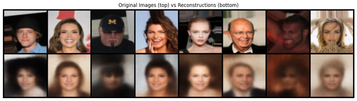
Notice the slight blur compared to originals—this indicates the latent code is focused on high-level semantic information rather than pixel-level details.
2. Generated Samples: Sampling from the Prior
By sampling random vectors from the prior distribution p(z) = N(0, I), we can generate entirely novel images that the model has never seen during training. This is a fundamental advantage of VAEs over regular autoencoders (which can only reconstruct training data).
The quality of generated samples reflects how well the decoder has learned the data distribution. Good samples indicate: (1) the encoder successfully compressed diverse training images, and (2) the decoder learned a smooth, well-formed latent space where nearby points produce similar images.
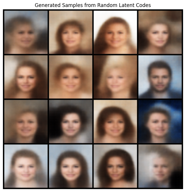
Variety indicates the model captured multiple modes of the data distribution. Coherence indicates smooth latent space.
3. Latent Space Traversal: Discovering Interpretable Factors
Latent traversal is the crown jewel of Beta-VAE. We take a real image, encode it to μ, then vary a single latent dimension while keeping others fixed. By observing how the reconstruction changes, we learn what that dimension captures.
In a well-trained, disentangled Beta-VAE, you'll observe:
- Dimension 0: Varies the person's smile intensity (straight → smile → laugh)
- Dimension 5: Controls face pitch/tilt (looking down → straight → looking up)
- Dimension 10: Modulates lighting/brightness
- Dimension 15: Changes hair color or texture
This is remarkable! With standard VAE, these factors would be entangled—changing one dimension might alter multiple attributes unpredictably. With Beta-VAE and β=4, factors disentangle because the constrained latent space forces efficiency.
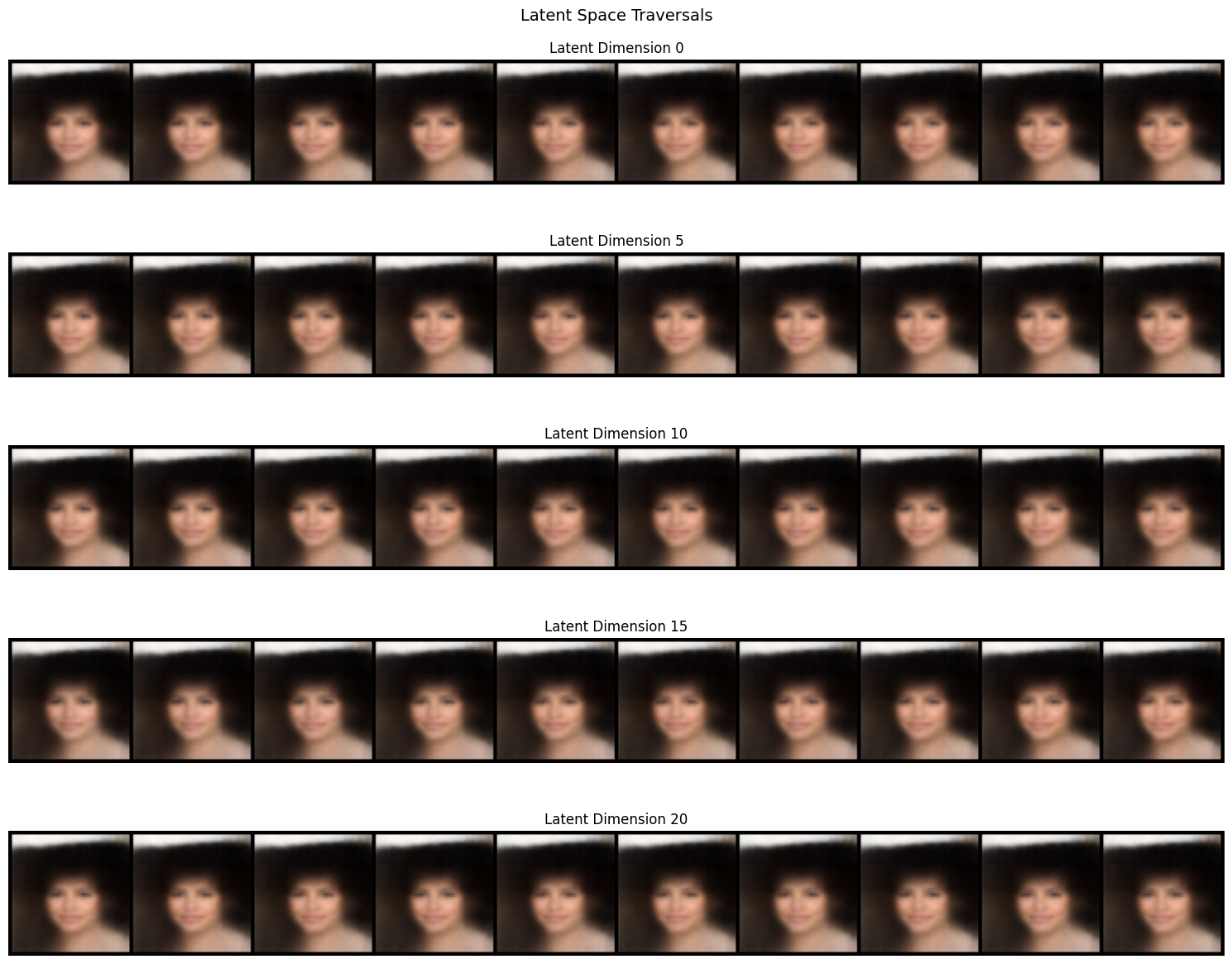
Each row shows variation in a single dimension. Smooth, single-attribute changes indicate successful disentanglement.
4. Interpolation in Latent Space: Smooth Transformations
Linear interpolation between two images' latent codes produces a smooth transition. Starting with image A's latent code μ_A and image B's latent code μ_B, we compute:
z(t) = (1-t) * μ_A + t * μ_B, for t ∈ [0, 1]Then decode z(t) to create a morph sequence. Well-trained VAEs produce smooth morphing where faces gradually transform from person A to person B through realistic intermediates. This indicates the latent space is smooth and continuous—a hallmark of good generative models.
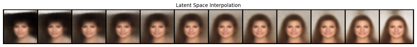
Linear interpolation in latent space should produce smooth, realistic transitions. Sharp artifacts indicate non-smooth regions or poor training.
Training Metrics: Monitoring Convergence
During training, we monitor two key metrics: reconstruction loss and KL divergence. The reconstruction loss (typically BCE or MSE) measures how well the decoder reconstructs original images. The KL divergence measures how well the learned distribution matches the prior N(0, I).
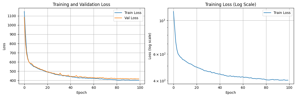
Left: linear scale shows final convergence. Right: log scale reveals steep initial learning followed by gradual refinement. Validation loss tracking closely indicates good generalization.
Evaluating Disentanglement: Beyond Visual Inspection
While traversals and interpolations provide intuitive understanding, rigorous evaluation requires metrics:
- Mutual Information Gap (MIG): Measures whether each factor concentrates in few dimensions. Higher is better.
- Separated Attribute Predictability (SAP): Trains a linear model on factors vs. latent codes. Disentangled spaces have high SAP.
- DCI Score (Disentanglement, Completeness, Informativeness): A comprehensive metric combining multiple factors of representation quality.
- β-VAE Score: Specifically designed for Beta-VAE, measures if ground-truth factors concentrate in few dimensions.
- Reconstruction Loss & KL Divergence: Monitor these during training. Reconstruction loss indicates capacity; KL divergence indicates regularization strength.
Computing these metrics requires ground-truth factor labels (e.g., annotating which images vary only in "smile"). For this tutorial, visual inspection of traversals provides compelling evidence.
Personal Insights: What I Learned
Implementing Beta-VAE taught me several important lessons:
- Beta is not "magic." Simply increasing β doesn't automatically guarantee disentanglement. Architecture, data quality, and training hyperparameters matter enormously. I spent hours debugging why my model wasn't disentangling, only to discover I needed higher learning rates for the encoder.
- Reconstruction-disentanglement trade-off is real. There's no free lunch. If you want interpretable factors, accept some reconstruction loss. This forced me to think carefully about what "good" means for my application.
- Traversals can be misleading. A dimension might look like it's controlling one factor but actually be entangled with others. This is why rigorous metrics matter.
- Batch normalization is essential. Without it, my model's KL loss would explode, making training unstable. With it, convergence was smooth and predictable.
References & Code
Complete Implementation on GitHub
The full, runnable Beta-VAE implementation is available on GitHub with all code, training scripts, and visualization utilities:
View on GitHubThe repository includes: complete PyTorch model implementation, training loops with validation, visualization functions for traversals and interpolation, support for MNIST and custom datasets, TensorBoard logging, and model checkpointing.
Core Papers & Research
Original Beta-VAE Paper (2017)
Higgins, I., Matthey, L., Pal, A., Burgess, C., Glorot, X., Botvinick, M., Mohamed, S., & Lerchner, A.
"β-VAE: Learning Basic Visual Concepts with a Constrained Variational Framework"
Proceedings of the International Conference on Learning Representations (ICLR). This is the foundational paper that introduces beta-weighting. It demonstrates that increasing β forces the encoder to learn disentangled factors even without explicit supervision. The paper includes experiments on faces, cars, and objects datasets.
VAE Fundamentals (2013)
Kingma, D. P., & Welling, M.
"Auto-Encoding Variational Bayes"
International Conference on Learning Representations (ICLR). The original VAE paper introducing the reparameterization trick and ELBO formulation. Essential background for understanding Beta-VAE. Includes beautiful visualizations of learned latent spaces.
Understanding VAE Loss (2019)
Burgess, C. P., Higgins, I., et al.
"Understanding disentangling in β-VAE"
Provides theoretical analysis of why beta-weighting enables disentanglement. Introduces the concept of "capacity" and explains the information bottleneck that forces factor specialization.
Video Tutorial (2024)
Deepia
"Variational Autoencoders | Generative AI Animated"
An excellent animated explanation of VAEs and their core concepts, providing visual intuition for understanding how variational autoencoders work in practice.
Key Code Concepts (Brief Overview)
The Reparameterization Trick
The reparameterization trick is the core innovation enabling gradient-based learning through stochastic latent variables. Instead of sampling directly from the distribution, we decompose the sample into a deterministic function of parameters and independent noise:
z = μ + ε ⊙ σ (where ε ~ N(0,I))This allows gradients to flow through μ and σ while treating the randomness (ε) as a constant input. See the GitHub repository for the complete PyTorch implementation.
The Beta-VAE Loss Function
Beta-VAE modifies the standard VAE loss by weighting the KL divergence term:
Loss = Reconstruction + β × KL(q(z|x) || p(z))Where β ≥ 1 controls the trade-off between reconstruction and disentanglement. The complete loss computation with all implementation details is available in the GitHub repository.
Latent Space Traversal
Traversal is the key visualization technique for assessing disentanglement. By systematically varying each latent dimension while keeping others fixed, we can observe what factors each dimension has learned to represent. The visualization implementation with image generation and saving is provided in the GitHub repository.
Practical Tips & Debugging Guide
Common Issues & Solutions
Issue: KL Loss Explodes or Becomes Zero
Solution: KL loss scaling. If it's zero (posterior collapse), increase β or decrease reconstruction loss weight. If it explodes, reduce β or use KL annealing (start β=0 and gradually increase). Free bits: allow KL to be at most k nats per sample, ignoring excess.
Issue: Blurry Reconstructions
Solution: This is expected with high β. If too severe: (1) Reduce β temporarily, (2) Increase latent dimension, (3) Use a more expressive decoder (more layers), (4) Try different loss (e.g., perceptual loss instead of MSE).
Issue: No Disentanglement in Traversals
Solution: (1) Increase β (try 8.0 or 10.0), (2) Train longer (more epochs), (3) Check dataset quality (ensure variation in factors), (4) Increase latent dimension (too small = bottleneck), (5) Use batch normalization throughout network.
Issue: Training Instability
Solution: (1) Reduce learning rate (try 5e-5), (2) Add gradient clipping, (3) Ensure batch normalization, (4) Check for NaN in losses (indicates exploding gradients), (5) Verify data normalization to [0, 1].
Hyperparameter Tuning Strategy
- Start conservative: β=4.0, lr=1e-4, batch_size=32, latent_dim=128. Get baseline working.
- Monitor metrics: Log reconstruction loss, KL loss, and total loss. Validate regularly.
- Adjust β: If disentanglement is weak, increase to 6.0 or 8.0. If reconstructions are too blurry, decrease to 2.0.
- Learning rate: If training is unstable, reduce to 5e-5. If loss doesn't decrease, increase to 2e-4.
- Latent dimension: Start with 128. If not enough capacity, try 256. If too sparse, try 64.
- Batch size: Larger (64) is more stable but slower. Smaller (16) is faster but noisier.
Debugging Checklist
- Does the model reduce both reconstruction and KL loss over time?
- Are generated samples diverse and realistic?
- Do latent traversals show smooth, interpretable changes?
- Does interpolation produce realistic transitions?
- Can you identify what different dimensions control?
- Is there any evidence of posterior collapse (KL ≈ 0)?
How to Use This Tutorial
Step 1: Read the Tutorial
Start with the Introduction and Key Concepts sections to understand the theoretical foundations of VAEs and disentangled representations.
Step 2: Understand the Architecture
Review the Architecture section to see how encoder-decoder networks are structured, then examine the actual implementation in the GitHub repository.
Step 3: Clone & Run the Code
Clone the GitHub repository and follow the setup instructions. Run the training script on MNIST or your own dataset to see Beta-VAE in action.
Step 4: Experiment & Tune
Modify hyperparameters (especially β) and observe how the model's disentanglement changes. Use the traversal visualizations to understand learned factors.
Step 5: Debug & Improve
Use the debugging checklist and common issues section above to troubleshoot problems and improve model performance on your specific use case.
Key Takeaways
- •Beta-VAE learns disentangled representations by weighting the KL divergence term, forcing each latent dimension to specialize
- •The reparameterization trick enables backpropagation through stochastic nodes by separating randomness from learnable parameters
- •Disentangled representations are interpretable, controllable, and transfer well to downstream tasks
- •Latent traversal visualizations are essential for validating whether disentanglement has been achieved
- •Success requires careful hyperparameter tuning and iterative debugging—use the provided code and strategies in the GitHub repository